Experiments with CIFAR10 - Part 1
Background
A while ago, I got introducted to the topics of Self-Supervised Learning and Representation Learning. For anyone interested in the topics, I highly recommend checking out the Deep Unsupervised Learning course from Pieter Abbeel and co. at Berkeley. There’s also a recent tutorial Representation Learning without labels from ICML 2020 which is quite nice. As I was catching up on the research, I came across the recent papers Bootstrap your own latent (BYOL) and Big Self-Supervised Models are Strong Semi-Supervised Learners (SimCLR v2). Both papers had interesting and innovative ideas. From BYOL there was the idea of efficient self-supervised learning without using contrastive examples, and from SimCLR v2 was the idea of using semi-supervised learning in combination with self-supervised learning. I was intrigued by these ideas, and decided to run a small little experiment of my own using the CIFAR100 and CIFAR10 datasets (compute limits constrained my dataset choices). I was super excited and started by setting up a baseline on CIFAR10 using Resnets. This didn’t turn out to be so trivial, and thus started a detour leading to this series of experiments with Cifar10. I eventually plan to get back to my original project, but I want to use this series of posts to highlight the experiments I performed as I dived deeper into Resnets and Cifar10.
In these experiments, I primarily use accuracy and loss to evaluate the performance of my options. Solely optimizing for accuracy is not always the right way to run Machine Learning projects for most practical purposes, but here I wish to show quick and easy ways to run different exepriments and set up reliable baselines. I consider these as starting points and no where close to the end product. I’ve used PyTorch as the framework of choice and Paperspace for running my notebooks on a GPU. I’ve tried to keep the secondary hyper-parameters fixed while running experiments on a particular hyper-param, model architecture, normalization layers, etc. (For eg, while trying out different Resnet architectures, I’ve tried to keep the optimizer, learning rate schedule, training budget, etc fixed.)
For the posts, I’ve assumed that readers are familiar with basic Deep Learning and Neural Networks, CNNs and Resnets, PyTorch, and the CIFAR10 dataset.
All my notebooks are hosted at https://github.com/hemildesai/cifar10-experiments.
Naive Beginnings
Initially when starting out, I thought this was going to be super easy and had some pre-conceived notions. Create a data loader for the dataset, write a train function, write an evaluate function, select the Categorical Cross Entroy Loss, select the ADAM or SGD with Momentum Optimizer, decay learning rate, import resnet and train for some epochs. When it’s done, the model should achieve 94% accuracy at the minimum. So, here it goes -
# Data loaders
train_ds, test_ds = cifar10(batch_size=128)

# Optimizer and LR schedule
optimizer = torch.optim.SGD(model.parameters(), lr=0.05, momentum=0.9, weight_decay=5e-4)
scheduler = torch.optim.lr_scheduler.MultiStepLR(optimizer, milestones=[25, 40], gamma=0.1)

# Loss
criterion = nn.CrossEntropyLoss()

# Model
model = torchvision.models.resnet18(num_classes=10)

# Train and Evaluate
train(train_ds, test_ds, optimizer, model, scheduler=scheduler, epochs=50)
Turns out it’s not so straightforward. I run this and I reach 85.83% accuracy. Here are the graphs for the training loop for a resnet18 -
At first glance, it doesn’t look so bad for 50 epochs. But considering the baseline for Cifar10 is 94% and also looking at the DAWN benchmark this doesn’t look so good. I bang my head a little more, and try a few different hyper-parameters, optimizers, schedules, etc, but it seems to be stuck around the 85-86% mark. Experienced ML practicioners will be quick to point out my mistake, so feel free to take a look at the code block above and find the mistake. In agadmator’s voice, for those of you who were able to do it, congratulations on finding that the mistake lies in the Model, and for those who want to enjoy the show let’s dive deeper.
Fixing the mistake
Let’s start by examining the model. If you run just model in a Jupyter cell, the initial part will look like -
ResNet(
  (conv1): Conv2d(3, 64, kernel_size=(7, 7), stride=(2, 2), padding=(3, 3), bias=False)
  (bn1): BatchNorm2d(64, eps=1e-05, momentum=0.1, affine=True, track_running_stats=True)
  (relu): ReLU(inplace=True)
  (maxpool): MaxPool2d(kernel_size=3, stride=2, padding=1, dilation=1, ceil_mode=False)
....
)
If you look closely, the conv1 and maxpool layers seem odd for a 32x32x3 image in Cifar10. Unfortunately for us, the Resnet implementation in PyTorch and most frameworks assume a 224x224x3 image from ImageNet as input. When the size of the image is so large, it makes sense to have a 7x7 kernel with a stride of 2 as the first layer. This is because the receptive field of a kernel in the image will be a lot smaller compared to a 32x32 image. A 7x7 kernel in a 32x32 image will cover ~5% of the image in the first layer itself compared to a 224x224 image where the kernel will cover only ~0.1%. Applying a max pool layer after will not make much difference for a 224x224 image, but it will lead to a huge loss of information for the 32x32 image. So, reducing the kernel size and removing the Maxpool layer should fix the issue. In practice (after looking around a bit and doing some experiments), a 3x3 kernel with a stride of 1 and a padding of 1 works best. This explanation is based on my understanding, so happy to discuss this further if something seems odd.
Here’s how the fix is implemented in a very handy gist by Joost van Amersfoort for Cifar10-
resnet = models.resnet18(pretrained=False, num_classes=10)
resnet.conv1 = torch.nn.Conv2d(
    3, 64, kernel_size=3, stride=1, padding=1, bias=False
)
resnet.maxpool = torch.nn.Identity()
In my notebooks, I directly made the change in the source code of Resnet cause the source code will be necessary for other experiments we will look at later.
Using this fix in the model in the initial code block, you should get to around ~94% accuracy. The lesson I learnt from this is to not rush into things instantly but take a moment to look at the dataset along with any other libraries or architectures that you’re just importing into your experiment and think about how they work together. Here are the graphs for one of the training loops for a resnet18 (You should be able to see the difference from the first figure if you look closely) -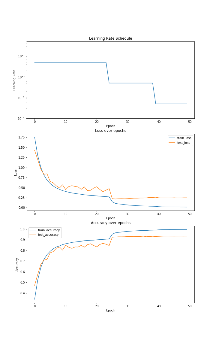
Messing with Normalization
While looking into BYOL and SimCLR v2, there was a lot of mentions and experiments on Batch Normalization and how batch size affects things. Compute constraints limit batch size, so methods that need a higher batch size become difficult with a smaller batch size. So I looked a bit deeper into normalization, and came across different normalization methods like batch, instance, group and layer. I also came across a paper on Weight Standardization which when combined with Group Normalization achieves similar performance as Batch Normalization even on micro batches. I was intrigued by this and decided to do a quick experiment using Resnets and Cifar10. Weight Standardization can be implemented as follows (taken from the official implementation at https://github.com/joe-siyuan-qiao/WeightStandardization ):
# Use this instead of nn.Conv2d at all places
class WeightStdConv2d(nn.Conv2d):
    def __init__(self, in_channels, out_channels, kernel_size, stride=1,
                 padding=0, dilation=1, groups=1, bias=True):
        super(Conv2d, self).__init__(in_channels, out_channels, kernel_size, stride,
                 padding, dilation, groups, bias)

    def forward(self, x):
        weight = self.weight
        weight_mean = weight.mean(dim=1, keepdim=True).mean(dim=2,
                                  keepdim=True).mean(dim=3, keepdim=True)
        weight = weight - weight_mean
        std = weight.view(weight.size(0), -1).std(dim=1).view(-1, 1, 1, 1) + 1e-5
        weight = weight / std.expand_as(weight)
        return F.conv2d(x, weight, self.bias, self.stride,
                        self.padding, self.dilation, self.groups)
Group Normalization has an official implementation in PyTorch. You can adapt it for Resnet as follows -
if norm_layer is None:
            norm_layer = nn.GroupNorm
        self._norm_layer = norm_layer
...
# Do this for all norm layers. First argument is the number of groups, so group factor is the number of channels in a group.
self.bn1 = norm_layer(self.inplanes//self.group_factor, self.inplanes)
Using these modifications in the model and re-running the training loop, you should get similar accuracy as the original resnet even while decreasing the batch size. I used a batch size of 32 in my notebook because I did not use parallelism and as a result lower batch size increased training times. I will look into parallel and efficient ways to train the model on a single GPU with smaller batch sizes. Here are the graphs for resnet18 with group norm and weight standardization -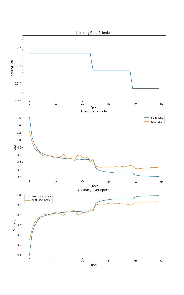
Conclusion
Cifar10 is a highly underrated dataset and an excellent one for running quick experiments and trying out a proof of concept for your ideas, especially if you are constrained by compute limits. That’s it for the experiments for part 1. In the next part, we’ll take a look at different learning rate schedules and also delve into a hidden gem in the toolbox - Stochastic Weight Averaging.