Introduction to Bayesian Inference

Foreword: The definitions and notations I’ve used in the post may deviate from the norm. I’ve used them in the form that has best helped me understand the concept. If you think that any of them is fundamentally wrong or if any citations are missing, please comment below or reach out to me and I’ll correct my mistakes.

Definitions

In the simplest of terms, Bayesian Inference is Inference using Bayes’ Theorem. Let’s define these individual components further:

Bayes’ Theorem

This is the equation we’re all familiar with:

$$ \large{P(A\mid{B}) = \frac{P(B\mid{A})P(A)}{P(B)}} \tag{1} $$

Inference

For the purpose of this post, let’s define the inference problem as follows:

Given a dataset $\mathcal{D} \sim {X,Y},\ X\ \in\ \mathbb{R}^{N\times Q},\ Y\ \in\ \mathbb{R}^{N\times D}$ consisting of $N$ inputs and observed outputs and a model $\mathcal{H}$ with parameters $\theta$, we want to learn $\theta$ from $\mathcal{D}$ in order to infer the output $y^*$, for some unseen input $x^* \notin\ \mathcal{D}$, such that it is closest to the real output $y^*_{true}$. In other words, we’re trying to learn a function $\mathcal{H}$ parameterized by $\theta$ from $\mathcal{D}$ such that

$$ \large\mathcal{H}_{\theta}(x^*) \approx y^*_{true} \tag{2} $$

Bayesian Inference

Now that we’ve defined Inference, let’s see how we can use Bayes’ Theorem to perform Bayesian Inference. We’ve established above that we need to learn the parameters $\theta$ of our model $\mathcal{H}$ from our dataset $\mathcal{D}$. But what does it mean to learn the parameters? How do we know that these learned parameters are good enough?

Since we’re dealing with probabilities here, let’s answer these questions with probabilities as below:

Let’s define the $Likelihood$ as $P(\mathcal{D}\mid\theta)$. Intuitively, this measures the goodness of fit for our model $\mathcal{H}$ given a particular set of $\theta$. This can help us answer how good these parameters explain the dataset $\mathcal{D}$.

Before starting to learn, we might have some beliefs or assumptions about the parameters. Let’s encode these as $P(\theta)$, calling it the $Prior$.

Once we’ve established the $Prior$ and the $Likelihood$, we can use equation $(1)$ to perform the learning step of Inference in the following manner:

$$ \large \underbrace{P(\theta \mid \mathcal{D})}_{Posterior} = \frac{\overbrace{P(\mathcal{D}, \theta)}^{Likelihood}\ \times \overbrace{P(\theta)}^{Prior}}{\underbrace{P(\mathcal{D})}_{Evidence}} \tag{3} $$

The $Evidence$ is the marginalized likelihood. It measures how well our chosen model $\mathcal{H}$ represents the data.¹

The $Posterior$ captures the distribution of our parameters given the data. Ideally, it should have peaks at values that have a high likelihod. This is what we need to perform the next step of Inference.

Given the $Posterior$, given $x^*$, we can predict $y^*$ as follows:

$$ \large P(y^*\mid{x^*, \mathcal{D}}) = \int{P(y^*\mid{x^*, \theta})}{P(\theta \mid \mathcal{D})}d\theta \tag{4} $$

With the distribution for $y^*$, we can calculate $E[y^*]\ or\ \mu_{y^*}$ as the predictive mean and $E[(y^* - E[y^*])^2]\ or\ \sigma_{y^*}^2$ as the predictive uncertainty.²

Bent Coin Problem

The rest of this post is about applying the steps of Bayesian Inference to the Bent Coin Problem. Along the way, we’ll also learn interesting things about the Bernoulli, Binomial and Beta distributions.

Problem Statement

Let’s assume we have a bent coin with the probability of landing heads as $\lambda$. We can observe $N$ number of coin tosses from the bent coin. Each coin toss can be expressed as a Bernoulli trial. If the outcome of the coin toss is represented by $y\in \{0,1\},\medspace 0 \rightarrow \text{Tails},\ 1 \rightarrow \text{Heads}$, then the probability of $y$ given the above biased coin can be expressed as:

$$p(y\mid \lambda) = \lambda^y(1 - \lambda)^{(1-y)} \tag{5}$$

This is also the likelihood of a single coin toss. If you think of $N$ coin tosses, the probability of $m$ heads then takes the form of a Binomial distribution as:

$$P(\mathcal{D}\mid\lambda,m) = \dbinom{N}{m}\lambda^m(1-\lambda)^{N-m}\qquad\mathcal{D}\in \{0,1\}^N \tag{6}$$

Note that, for inference, we’re trying to predict $\lambda$ so that we can then consequently predict the probability that the next coin toss is a head. So, our model here is just the distribution of $\lambda$(that’s all we need to predict) and the model parameter is just $\lambda$.

Prior Selection

In order to perform Bayesian Inference, we need to put a prior on $\lambda$, which is a probability. A very common distribution on probabilities is the Beta distribution defined below:³

$$ \begin{aligned} P(\lambda)& = \mathcal{Beta}(\lambda;\alpha, \beta) &\lambda \in [0,1] \\ \\ & = \frac{\lambda^{\alpha-1}(1-\lambda)^{\beta-1}}{\mathcal{B}(\alpha,\beta)} &\mathcal{B}(\alpha,\beta)\text{ is called the Beta function} &\hspace{8em} (7) \\ \\ \mathcal{B}(\alpha,\beta)& = \int_0^1{\lambda^{\alpha-1}(1-\lambda)^{\beta-1}}d\lambda && \\ \\ & = \frac{\Gamma(\alpha)\Gamma(\beta)}{\Gamma(\alpha+\beta)} &\Gamma(\alpha)\text{ is called the Gamma function} &\hspace{8em} (8) \\ \\ \Gamma(\alpha)& = (\alpha-1)!&&\hspace{8em} (9) \end{aligned} $$

Let’s take a look at how this distribution looks under different values of $\alpha$ and $\beta$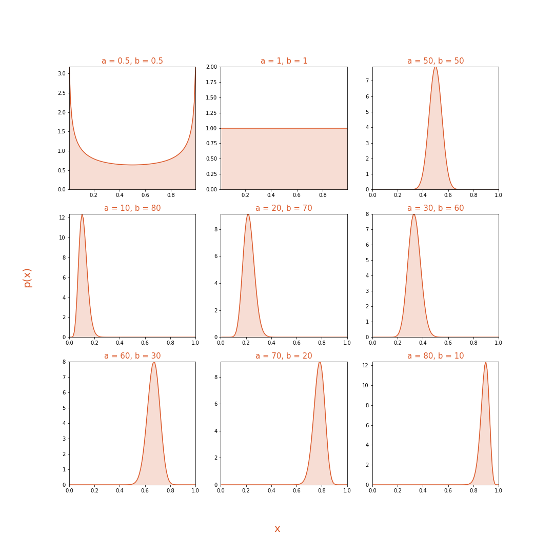

The Beta distribution also has one very useful property in the context of this problem. Techincally, the Beta prior is called the Conjugate Prior to the Likelihood function. This means that the posterior distribution will have the same form as our prior. This property will make it a breeze to calculate our posterior analytically.

Posterior

We have the prior and the likelihood, so let’s calculate the posterior (for a given $m$). Applying $eq\ (3)$ we get

$$ P(\lambda\mid\mathcal{D}) = \frac{P(\mathcal{D}\mid\lambda)P(\lambda)}{P(\mathcal{D})} \tag{10} $$

First, let’s evaluate the evidence or the marginal likelihood $P(\mathcal{D})$:

$$ \begin{aligned} P(\mathcal{D}) &= \int{P(\mathcal{D}\mid\lambda)P(\lambda)}d\lambda \\ \\ &= \int{\Bigg(\dbinom{N}{m}\lambda^m(1-\lambda)^{N-m}\times\frac{\lambda^{\alpha-1}(1-\lambda)^{\beta-1}}{\mathcal{B}(\alpha,\beta)}\Bigg)}d\lambda\qquad&\text{from eq (6) and (7)} \\ \\ &= \dbinom{N}{m}\frac{1}{\mathcal{B}(\alpha,\beta)}\int{\lambda^{m+\alpha-1}(1-\lambda)^{N-m+\beta-1}d\lambda} \\ \\ &= \dbinom{N}{m}\frac{\mathcal{B}(m + \alpha,N - m + \beta)}{\mathcal{B}(\alpha,\beta)}\qquad&\text{from eq (8)}&\hspace{2em}(11) \end{aligned} $$

Next, let’s plug in the values in $(10)$

$$ \begin{aligned} P(\lambda\mid\mathcal{D}) &= \frac{\bcancel{\dbinom{N}{m}}\lambda^m(1-\lambda)^{N-m}\times\frac{\lambda^{\alpha-1}(1-\lambda)^{\beta-1}}{\bcancel{\mathcal{B}(\alpha,\beta)}}}{\bcancel{\dbinom{N}{m}}\frac{\mathcal{B}(m + \alpha,N - m + \beta)}{\bcancel{\mathcal{B}(\alpha,\beta)}}} \\ \\ &= \frac{\lambda^{m+\alpha-1}(1-\lambda)^{N-m+\beta-1}}{\mathcal{B}(m + \alpha,N - m + \beta)} \\ \\ &= \mathcal{Beta}(\lambda;m+\alpha,N-m+\beta)&\hspace{16.5em}(12) \end{aligned} $$

We see that the posterior is also the Beta distribution, which is why our prior is called a conjugate prior above. This also gives an intuition about what $\alpha$ and $\beta$ represent in our prior. We can think of them as a prior run of the coin which yielded $\approx$ $\alpha - 1$ heads and $\beta - 1$ tails. As we observe another run with $N$ tosses and $m$ heads our prior gets updated as shown above. For yet another subsequent run, the above posterior now becomes the prior. This is one of the reasons why I love this example, it engrains the concepts of Bayesian Inference nicely into one’s mind.

Prediction

Now onto the second step of inference. Using $eq (4)$ we get

$$ \begin{aligned} P(y^* \mid \mathcal{D}) &= \int{P(y^*\mid\lambda)P(\lambda\mid\mathcal{D})d\lambda} \\ \\ &= \int{\lambda^{y^*}(1 - \lambda)^{(1-y^*)}\times\frac{\lambda^{m+\alpha-1}(1-\lambda)^{N-m+\beta-1}}{\mathcal{B}(m + \alpha,N - m + \beta)}d\lambda} \\ \\ &= \begin{cases} \large\frac{m + \alpha}{N+\alpha+\beta}\qquad &\text{if } y^*=1 \\ \\ \large\frac{N - m + \beta}{N+\alpha+\beta}\qquad &\text{if } y^*=0 \end{cases}&\hspace{10.5em}(13) \end{aligned} $$

This should be easy to show by using the above equations of the Beta and Gamma functions. Note that the mean of our posterior is also $\frac{m + \alpha}{N+\alpha+\beta}$. So, for our predictive point estimate, we’re performing what’s called a Bayesian Model Average (BMA)⁴ over the posterior.

Practical Example

Let’s take a look at the entire process in practice. We’ll take a look at two examples. For both examples, we set the true probability of heads ($\lambda$) to $0.80$.

1. For the first example, we’ll select a uniform prior (this can be done by setting both $\alpha$ and $\beta$ to $1$). We’ll proceed through 100 random coin tosses from the bent coin with $\lambda=0.80$. After each toss, we’ll calculate the new posterior. Then we’ll combine these posteriors in this video (shown below) to see how the posterior changes over time.

   Your browser doesn’t support embedded videos, but don’t worry, you can download it and watch it with your favorite video player!

2. For the second example, we’ll select a prior biased in the opposite direction ($\alpha = 1,\ \beta = 5$). We’ll see the posterior change over 250 coin tosses in this example. We’ll see that even if we have a prior biased in the opposite direction, the posterior distribution will eventually get to the point where it’s mode is equal to the true $\lambda$.

   Your browser doesn’t support embedded videos, but don’t worry, you can download it and watch it with your favorite video player!

I hope this gives a good intuition for the entire Bayesian Inference process. I’d appreciate any feedback and constructive criticism.

Further Learning

There are plenty of wonderful resources including books, courses, lectures, notes, etc out there to learn about Probabilistic Machine Learning and Bayesian Inference. I’m going to share a few which I’ve gone through recently and have found helpful. I first came across this example in Andrew Gordon Wilson’s talk on Bayesian Neural Nets. Yarin Gal’s pair of talks on Bayesian Deep Learning are also a great resource to get started with Bayesian Inference specifically in the context of Deep Learning. You can find the videos here - Part 1 and Part 2. David MacKay’s course on Information Theory, Pattern Recognition and Neural Nets is still evergreen. I’ll end with one last resource - an in-depth course on Probabilistic Machine Learning by Philipp Hennig which is currently ongoing for the Summer 2020 session.