LitSurvey - Making Pre-trained Language Models Better Few-shot Learners
Introduction
Self-Attention, Transformers and Language Models have become ubiquitous in the world of Natural Language Processing ever since the paper Attention is all you need came to the forefront. Pre-trained language models, using the transformer architecture, have seen a steady rise in performance as well as size, with GPT-3 hitting the peak at 175 Billion parameters. These models have also shown tremendous performance on downstream tasks via fine-tuning, with BERT being the most famous one. This has massive implications for real world NLP tasks, since not everyone can train a pre-trained LM from scratch, but everyone can fine-tune on a downstream task in just a few lines of code. (See the revolutionary Transformers library which makes it a piece of cake). 1
Taking this a step further, GPT series has shown that large language models are also suitable for zero-shot and few-shot learning, where you just pre-pend annotated examples to the input prompt and the language model produces the correct output for a variety of tasks. See this example of few shot learning via GPT 3
few shot learning in @elicitorg. here's a demo showing what gpt3 returns for these statements untrained, then what it returns after just 5 training examples. takes minutes to add new task to elicit. no code required. pic.twitter.com/BfMJgtiXQk
— Jungwon (@jungofthewon) February 6, 2021
However, using 175 Billion parameter models is not suitable in most practical scenarios. So, the paper LMBFF tries to develop novel strategies for few-shot learning on medium sized language models. Their approach comprises of two primary strategies:
- Prompt based fine-tuning and automatic prompt generation
- Dynamically and selectively incorporating demonstrations into each prompt’s context
Prompt based fine-tuning
In naive terms, a prompt is the input sequence to a language model. Prompt based prediction involves treating the downstream task as a Language Modeling problem, where you incorporate the task’s context into the prompt and use the token predicted by the language model as a prediction of the downstream task. This is done by designing the prompt in an innovative way, a form of art that requires both domain expertise and the inner workings of the model. The authors suggest using prompt-based prediction for fine-tuning, and also suggest a novel method to automatically generate prompts.
Incorporating demonstrations
GPT3 achieves few shot learning by including annotated examples from the downstream task directly into the prompt along with the sequence to predict on. It does so without changing the underlying weights of the model. The annotated demonstrations are included in a naive way by simply concatenating randomly sampled examples. The authors develop a more refined sampling strategy that creates multiple sets including one example from each class as well as picking examples more relevant to the input sequence.
The authors observe the following results:
- Prompt-based fine-tuning largely outperforms standard fine-tuning
- Our automatic prompt search matches or outperforms manual prompts
- Incorporating demonstrations is effective for fine-tuning, and boosts few-shot performance
Here’s a quick summary from the authors themselves
Excited to share a preprint, “Making Pre-trained Language Models Better Few-shot Learners”!
— Adam Fisch (@adamjfisch) January 2, 2021
GPT-3's huge LM amazingly works directly for few-shot learning. We take things further, and propose fine-tuning techniques to make smaller LMs work better too.https://t.co/iIQf3ND4hE pic.twitter.com/Bt2t66w5EX
Now, let’s dive into the technical details.
Some Technical Deets
$$ \begin{aligned} \mathcal{L} \rightarrow& \text{ represents the pre-trained Language Model} \\ \mathcal{D} \rightarrow& \text{ represents the dataset for the downstream task we want to fine-tune on} \\ \mathcal{Y} \rightarrow& \text{ represents the label space for } \mathcal{D} \\ K \rightarrow& \text{ represents the number of training examples per class } \\ K_{tot} =& \:K \times \mid{\mathcal{Y}}\mid \\ \mathcal{D_{train}} =& \:\{x_{in}^i,y^i\}_{i=1}^{K_{tot}} \\ \mathcal{D_{test}} \sim& \:(x_{in}^{test},y^{test}) \:\text{ represents the unseen task set} \\ \mid{\mathcal{D_{dev}}}\mid =& \: K_{tot} \:\text{ represents the dev set} \end{aligned} $$
For most experiments the authors use $\mathcal{L} =$ RoBERTa-large and $K = 16$.
Datasets
- Single-sentence tasks $<S_1>$ - Tasks include sentiment analysis, question classification and grammaticality assessment.
- Sentence-pair tasks $(<S_1>,<S_2>)$ - Tasks include natural language inference, paraphrase detection and relation prediction.
Evaluation
Fine tuning on small datasets often suffer from instability. Hence, for every experiment, the authors measure average performance across 5 different randomly sampled $\mathcal{D_{train}}$ and $\mathcal{D_{dev}}$ splits, using a fixed set of seeds $\mathcal{S_{seed}}$. This improves the model’s robustness. The authors also do a grid search over the hyper-parameters to find the best set for the dev dataset.
How Classical Fine-tuning works
For classical fine-tuning in MLM (masked language modeling) on a downstream classification task, you take the output representations of the special [CLS] token and train a new softmax head like $$ \text{softmax}(W_o h_{[CLS]}) $$ For a regression task, you just remove the softmax. During learning, you tune the parameters of $\mathcal{L}$ as well as $W_o$. For models like RoBERTa, a new $W_o$ can be substantial (2048 new parameters for a binary classification task). This makes it unstable for few-shot learning where there’s not enough data to tune the parameters.
Here’s an image from the paper which sums up the process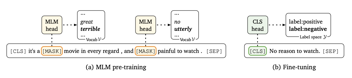
How Prompt based Fine-tuning works
In prompt based fine-tuning, $\mathcal{L}$ is directly tasked with predicting the downstream task. This is done by designing the prompt in such a way that when $\mathcal{L}$ autocompletes the prompt, the result is what we need. For instance, if we have a binary sentiment classification task, we can design the prompt as: $$ x_{\text{prompt}} = \text{[CLS] }x_1\text{. It was [MASK]. [SEP]} $$
Now if $\mathcal{L}$ predicts something like “awesome” or “amazing”, we can assume the sentiment is positive. Whereas if it predicts “terrible”, we can assume the sentiment is negative. Let’s see how this works for classification and regression.
Classification
For classification, you basically map the output of the language model to the labels of the downstream task and try to tune the params. You modify the input sequence to a clever designed prompt with one [MASK] token such that $\mathcal{L}$'s output representation for [MASK] is closest to the word that maps to the correct label. You can get a distribution by taking the softmax over the inner product of the output representation and the word vector obtained in pre-training as
$$
\begin{aligned}
p(y \mid x_\text{in}) &= p([\text{MASK}] = \mathcal{M}(y)\mid x_\text{prompt})
\\ &= \frac{\exp{(w_{\mathcal{M}(y)} \times h_\text{[MASK]})}}{\sum_{y^{'}\in\mathcal{Y}}\exp{(w_{\mathcal{M}(y^{'})} \times h_\text{[MASK]})}}
\\ \\ & \mathcal{M}: \mathcal{Y} \rightarrow \mathcal{V} \text{ denotes the injective mapping from labels to words produced by } \mathcal{L}
\\ & h_\text{[MASK]} \text{ denotes the output representation for [MASK] from } \mathcal{L}
\\ & w_v \text{ denotes the pre-softmax output vector for any word used in pre-training } v \in \mathcal{V}
\end{aligned}
$$
$\mathcal{L}$ can be fine-tuned to minimize cross entropy for the training set. The process is visualized below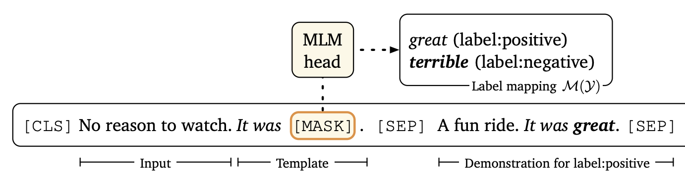
“No reason to watch.” is the input sequence $x_in$ which is transformed to the prompt $x_\text{prompt}$ “[CLS] No reason to watch. It was [MASK]. [SEP]". The transformation function is denoted by $\mathcal{T}$ and is called the template. We’ll talk about the demonstrations in a later section.
Regression
For regression, we bound the label space in an interval on the real line. For instance, we can formulate a binary sentiment classification task as a regression problem ranging from 0(terrible) to 1(amazing). Then the prediction can be a mixture model which is basically a weighted sum of 0 and 1. The two probabilities (for 0 and 1) sum up to 1 and can be predicted in the same way as for a classification task. This post will mainly focus on classification, but you can look into the paper for further details about regression.
All about Prompts
The template $\mathcal{T}$ and the label words $\mathcal{M}(\mathcal{Y})$ together can be called the prompt $\mathcal{P}$. For the binary sentiment classification task
$$
\mathcal{T}(x_{in}) = x_{in} + \text{“It was [MASK]. [SEP]"}
\\ \mathcal{M}(\mathcal{Y}) \rightarrow \text{\{great, terrible\}}
$$
This is a manually designed prompt. Designing this is a work of art, requiring domain expertise and trial and error. It may seem trivial for simple tasks, but can get complicated very quickly. Additionally, prompt design can have a massive impact on performance. Just look at this pilot study from the paper -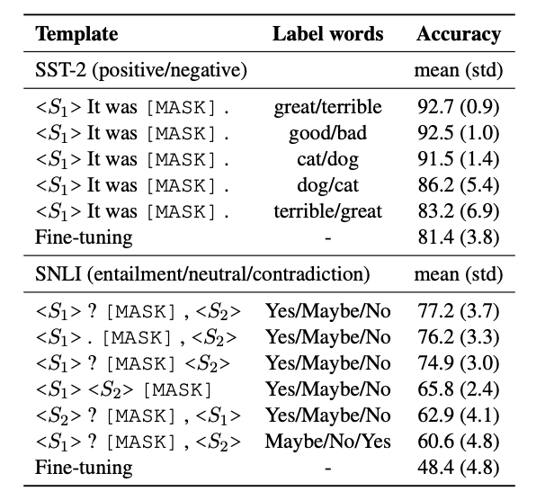
Automatic Prompt Generation
Wouldn’t it be great if we have an oracle that tells us the most efficient prompt? Designing such an oracle is a tough challenge though. You can imaging the search space we’d have to go through. To combat this, the authors propose a principled approach to automating the search process.
Automatic selection of Label Words
This involves developing $\mathcal{M}$ given $\mathcal{T}$. To do this, the authors use the inductive biases of $\mathcal{L}$. For each class $c \in \mathcal{Y}$, you pass all its examples through $\mathcal{T}$, and then pass each prompt to $\mathcal{L}$. Then you take the top-k probabilities for the [MASK] token output by $\mathcal{L}$ across all the examples and use it as $\mathcal{V}^c$. We then find the top-n assignments based on $\mathcal{D}_\text{train}$. Next, you re-rank and fine-tune all n assignments to find the best one on $\mathcal{D}_\text{dev}$. Doing this for all classes gives the complete mapping $\mathcal{M}(\mathcal{Y})$.
Automatic generation of templates
As you may have guessed, this involves developing $\mathcal{T}$ given $\mathcal{M}$. For this, we use the T-5 model. One of the pre-training objectives of T5 is to complete phrases. For example, given “Thank you <X> me to your party <Y> week”, T5 is trained to predict “for inviting” for <X> and “last” for <Y>. Let’s see how we can use this for templates. Given an input training example $(x_{in},y) \in \mathcal{D_\text{train}}$, we denote conversions $\mathcal{T_g}(x_{in},y)$ as
$$
<S_1>\quad \rightarrow \quad<X> \mathcal{M}(y) <Y> <S_1>
\\ <S_1>\quad \rightarrow \quad<S_1> <X> \mathcal{M}(y) <Y>
\\ <S_1>, <S_2>\quad \rightarrow \quad<S_1> <X> \mathcal{M}(y) <Y> <S_2>
$$
<X> and <Y> are predicted by T5. For generating $\mathcal{T}$, the goal is to find an output that works for all examples in the training set. This can be done by maximizing the log probability of the templates (combination of the predictions of T5). Beam search with a wide beam width (100) is used to decode multiple candidates. The candidates are fine tuned on the train set and the best one (or top-k) is picked from the dev set. This process is illustrated below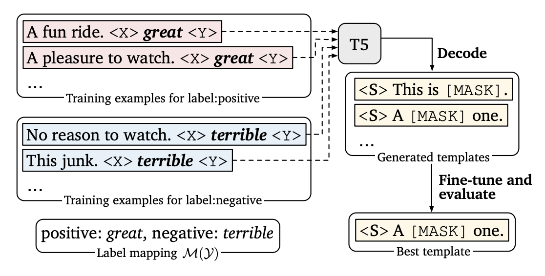
You may think this is a chicken and an egg problem picking between label words and templates, so we’ll discuss what the authors do to address that in a later section.
Incorporating Demonstrations
As we saw in the GPT3 example above, incorporating examples/demonstrations in the prompt can greatly improve performance. In GPT3, the annotated demonstrations are included in a naive way by simply concatenating randomly sampled examples. The authors study smart ways to do this for medium sized $\mathcal{L}$s.
Including training examples
At each step, the authors randomly sample one example from each class, transform that example using $\mathcal{\hat{T}}$, and concatenate them with the input. Given $x$ as “A fun ride” and $y$ as positive, $\mathcal{\hat{T}}(x,y) =$ “A fun ride. It was great.” The final prompt is given as $$ \mathcal{T^*}(x_{in}) = \mathcal{T}(x_{in}) \; \oplus \; \mathcal{\hat{T}}(x_{in}^1,y^1) \; \oplus \; ……. \; \oplus \; \mathcal{\hat{T}}(x_{in}^{|\mathcal{Y}|},y^{|\mathcal{Y}|}) $$ The authors sample multiple such demonstration sets. During training, they use one step per example. During inference, they ensemble across the sets.
Including demonstrations similar to the input
If the examples in the demonstration set are very different from each other or very different from the input sequence, the performance can be negatively impacted. To address this, the authors only sample examples close to the input. They do this by using Sentence-BERT. This gives the sentence embeddings for each sequence. The authors only consider the top 50% of samples similar to the input measured by their cosine similarity.
Takeaways
The key takeaways can be best summarized by the tables in the paper. The authors compare their approach to standard classical fine-tuning, fine-tuning on the entire parent training set, a majority baseline where you just predict the most frequent class, zero-shot learning and GPT3 style “in-context” prediction with demonstrations. Massive improvements are seen on all tasks, summarized by this table below (auto and man refer to automatic and manual prompt generation)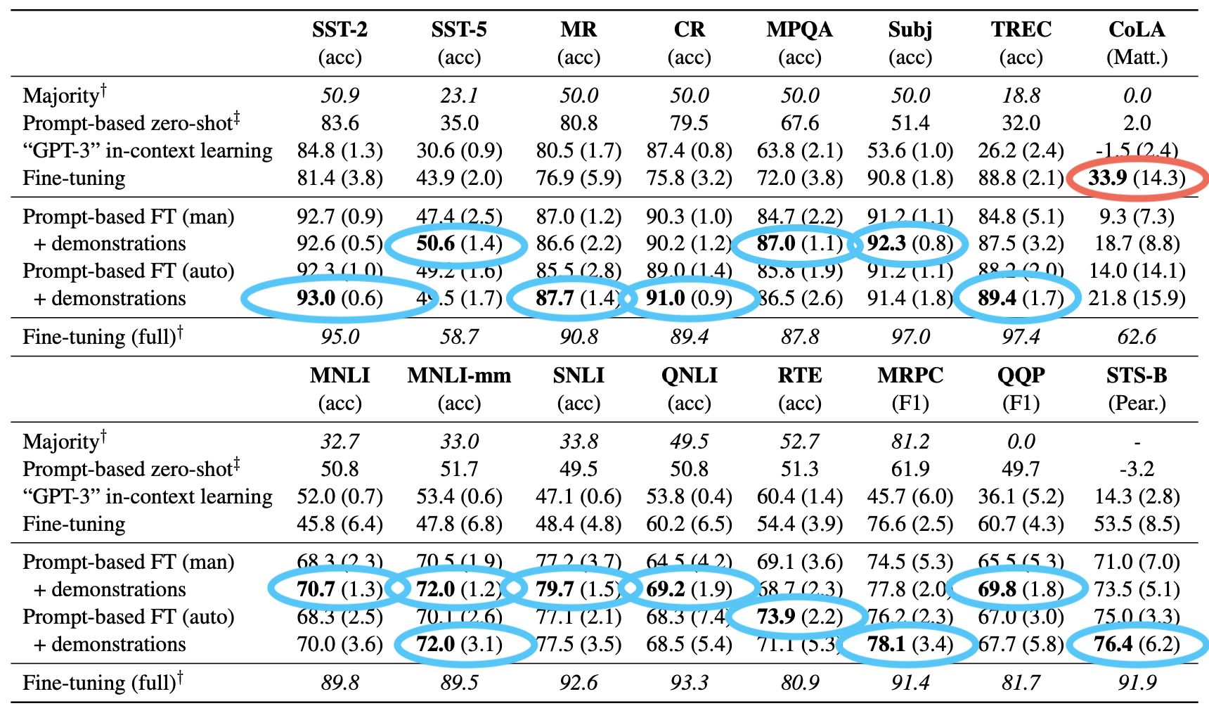
Ensembles
Using ensembles help in most cases, and this is no exception. The authors form ensembles by selecting a group of automatic prompts. They compare them with a group of manual prompts. The results are as follows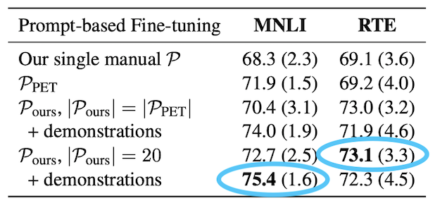
Automatic Prompts
Remember the chicken and egg problem in automatic prompts? The authors deal with it in three ways:
- Generate labels using manual templates (Auto L)
- Generate templates using manual labels (Auto T)
- Joint variant, generate one after the other starting from manual labels (Auto L+T)
Let’s take a look at the result as well as some generated prompts.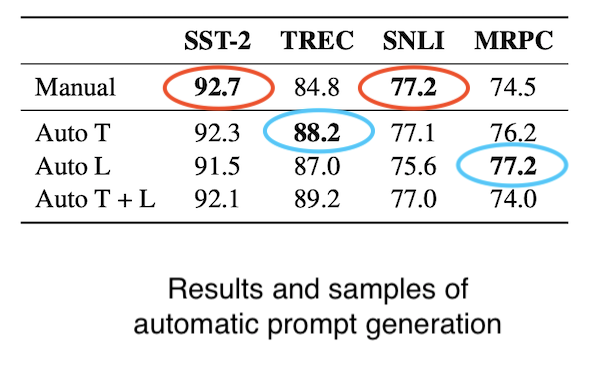
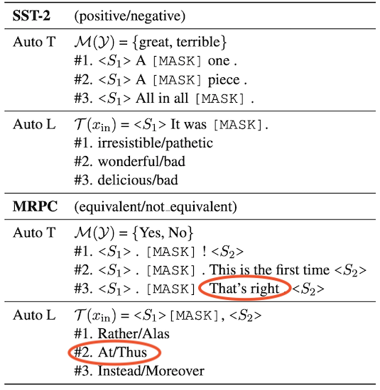
The results look comparable at the very least, and better in two tasks. The samples look mostly reasonable, with the exception of some bias and irregularities highlighted in red.
Incorporating Demonstrations
Uniform sampling of demonstrations combined with sentence similarity also leads to gains in results. Since SentenceBERT is trained on SNLI and MNLI, the authors also experiment with a mean pooling encoder using RoBERTa-large.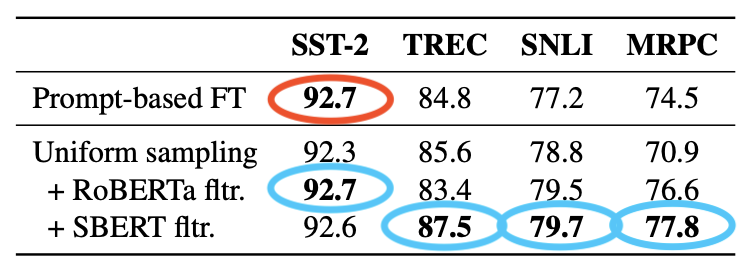
Sampling efficiency
The best way to summarize this is by looking at the plots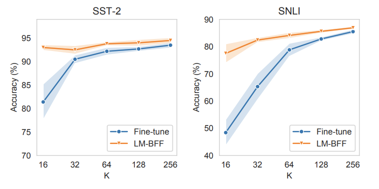
The plots show that for a few-shot setting when the number of examples per class is limited, LM-BFF vastly outperforms classical fine-tuning. However, classical fine-tuning seems to catch-up as the number of examples increase. Still LM-BFF seems to work pretty well even with higher number of examples per class.
Related Work
GPT Series
The development of prompt based few shot learning has been fueled by the GPT series (GPT, GPT 2, GPT-3). Specifically, GPT-3 showed amazing results on few shot learning, as illustrated by the tweet shared at the beginning of the post. The paper develops on the key concepts of GPT-3 - prompting and in-context learning, and adapts it to medium sized Masked Language Models since using 175 billion parameters is not pragmatic in most settings.
PET
The PET paper focuses on a semi-supervised setting in which a large set of unlabeled examples are provided. They use the prompt based approach to generate a soft labeled dataset. Basically, they run the unlabeled examples through the prompt templates in a pre-trained language model and use the predictions to generate soft labels. This works great for a semi-supervised training approach. The prompt based templating is very similar between PET and LM-BFF.
Fine-Tuning approaches
Papers like Fine-Tuning Pretrained Language Models: Weight Initializations, Data Orders, and Early Stopping develop better and more efficient fine-tuning methods building on top of the classical fine-tuning pipeline. They do so by improving optimization and regularization techniques to stabilize fine-tuning on a smaller dataset compared to the larger dataset used in pre-training. In LM-BFF, the authors use standard optimization and regularization techniques and focus their efforts on prompt-based fine-tuning.
Meta-Learning
Meta-learning approaches for few shot learning like LEOPARD use optimization based meta-learning with the hope to achieve generalization across a diverse set of NLP tasks. This meta learning helps achieve good performance on tasks never seen during training, with as few as 4 examples per class. While this can also be considered as few-shot learning, LM-BFF differs in the sense that they do not use any sort of meta-learning.
Intermediate Learning
In recent work like UFO-ENTAIL, the authors pre-train an entailment model, and use it on new downstream entailment tasks in a few shot setting. This differs from LM-BFF in the sense that it uses an intermediate entailment dataset to pre-train an entailment model on top of the language model. However, LM-BFF does not use any intermediary tasks or datasets and just directly uses the few-shot dataset itself.
Conclusion
LM-BFF can be summed up as a set of tools that help achieve great performance for downstream tasks with a few-shot setting. The code for the paper can be found at https://github.com/princeton-nlp/LM-BFF. It would be amazing to see integrations of LM-BFF with popular libraries like transformers so that the tools can be easily used in real world applications.
To learn more about transformers and language models, check out the blog posts at https://jalammar.github.io/ ↩︎